library(tidyverse)
library(cowplot)
library(calendR)Assignment Habits - Intro to R Class Summer 2025
Packages Used
Reading in CSV file and Checking Out Data
data <- read.csv('IntroToR-SubmissionsDecodedMasked-07282025.csv')Tidying and Cleaning
- Seperating datetime to date and time, seperate columns
- Cast date variable as Date
- Turn course name to factors
data <- data %>% separate_wider_delim(datetime, " ", names = c("date", "time"))
data$date <- as.Date(data$date)
data$course_name <- factor(data$course_name, levels = c('R Programming', 'Exploratory_Data_Analysis'))
Quick Glimpse
glimpse(data)Rows: 7,152
Columns: 9
$ course_name <fct> Exploratory_Data_Analysis, Exploratory_Data_Analysis, …
$ lesson_name <chr> "Principles_of_Analytic_Graphs", "Principles_of_Analyt…
$ question_number <int> 3, 7, 11, 14, 21, 21, 21, 25, 32, 33, 34, 35, 37, 3, 5…
$ correct <lgl> TRUE, TRUE, TRUE, TRUE, FALSE, FALSE, TRUE, TRUE, TRUE…
$ attempt <int> 1, 1, 1, 1, 1, 2, 3, 1, 1, 1, 1, 1, 1, 1, 1, 1, 1, 1, …
$ skipped <lgl> FALSE, FALSE, FALSE, FALSE, FALSE, FALSE, FALSE, FALSE…
$ date <date> 2025-07-14, 2025-07-14, 2025-07-14, 2025-07-14, 2025-…
$ time <chr> "23:28:00.44013", "23:29:13.22424", "23:29:54.15472", …
$ student_id <int> 1, 1, 1, 1, 1, 1, 1, 1, 1, 1, 1, 1, 1, 1, 1, 1, 1, 1, …Looking at Class Data All Together
#Attempts by Question for each course-lesson
data |>
  ggplot(aes(x=question_number, y=attempt)) +
  geom_col() +
  facet_wrap(course_name~lesson_name, scales='free') +
  theme_cowplot() +
  theme(strip.text.x = element_text(size = 8)) +
  labs(x='Q #', y='# Attempts')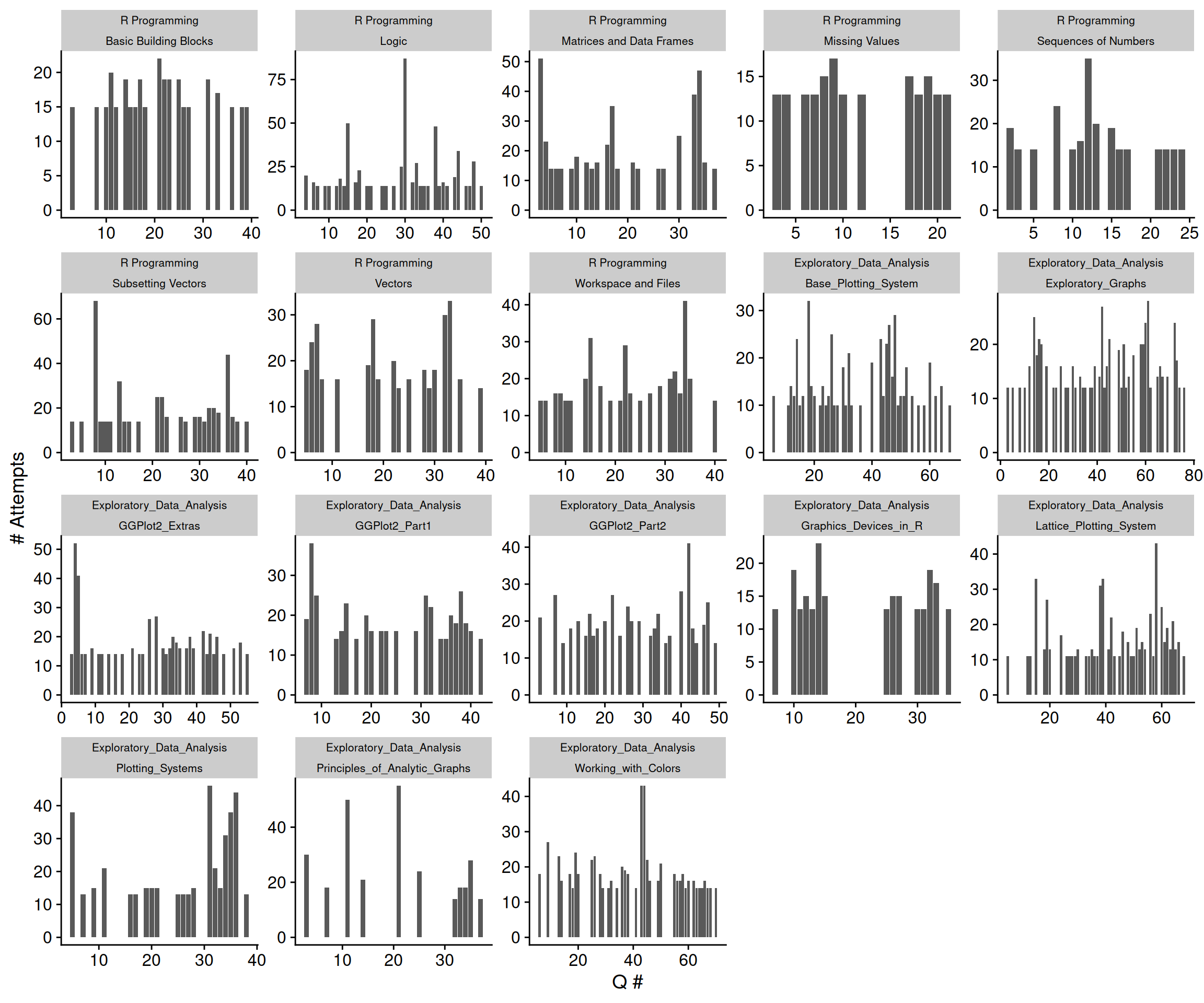
#Dates they were completed
data |>
  ggplot(aes(x=date, y=attempt)) +
  geom_col() +
  scale_x_date(date_breaks = "1 day" , date_labels = "%b %d") +
  facet_wrap(course_name~lesson_name, scales='free') +
  theme_cowplot() +
  theme(axis.text.x = element_text(angle=90, hjust=1), strip.text.x = element_text(size = 8)) +
  labs(x='Date', y='# Attempts')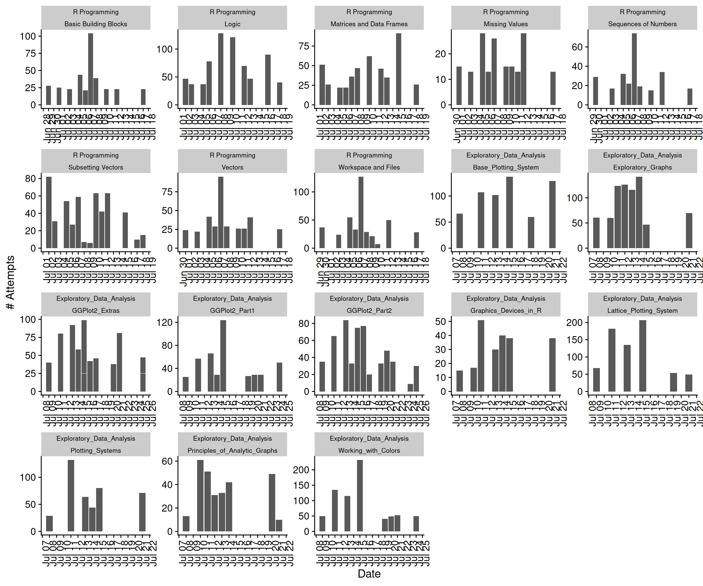
#Heatmap of dates lessons were completed
calendar_df_all <- data %>% count(date)
days_all <- calendar_df_all$n
days_all <- c(days_all, rep(0,8))

calendR(from = "2025-06-29",
        to = "2025-07-30",
        special.days = days_all,
        gradient = TRUE,
        low.col = "white",
        special.col = "#FF0000")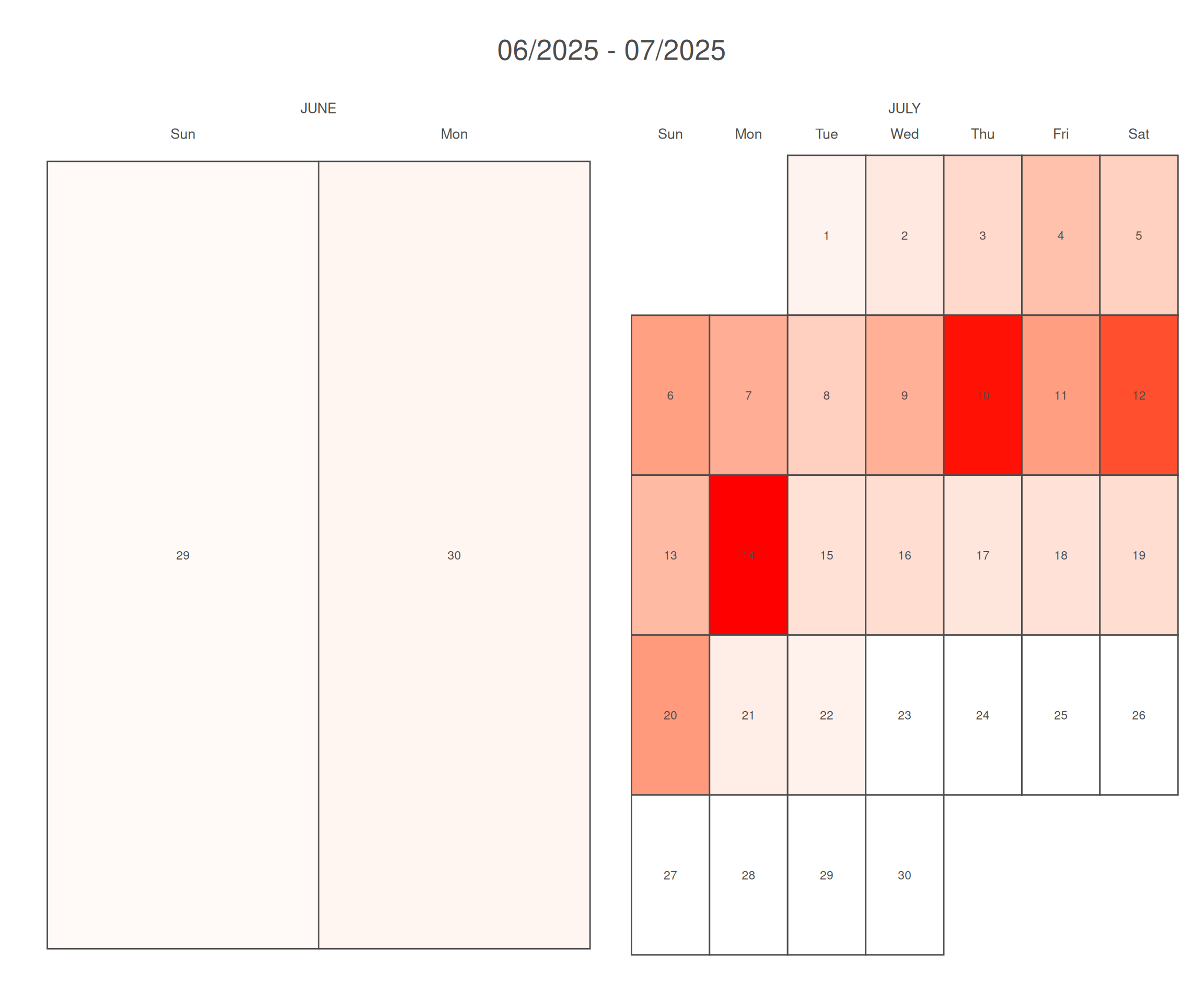
#Late start on the first assignment and early start on the second #Look a the hour of the day they are completed
data |>
ggplot(aes(x=as.POSIXct(time, format="%H:%M"), y=attempt)) +
geom_col() +
scale_x_datetime(
date_breaks = "5 hour",
date_labels = "%H:%M") +
facet_wrap(course_name~lesson_name, scales='free') +
theme_cowplot() +
theme(axis.text.x = element_text(angle=90, hjust=1), strip.text.x = element_text(size = 8)) +
labs(x='Time', y='# Attempts')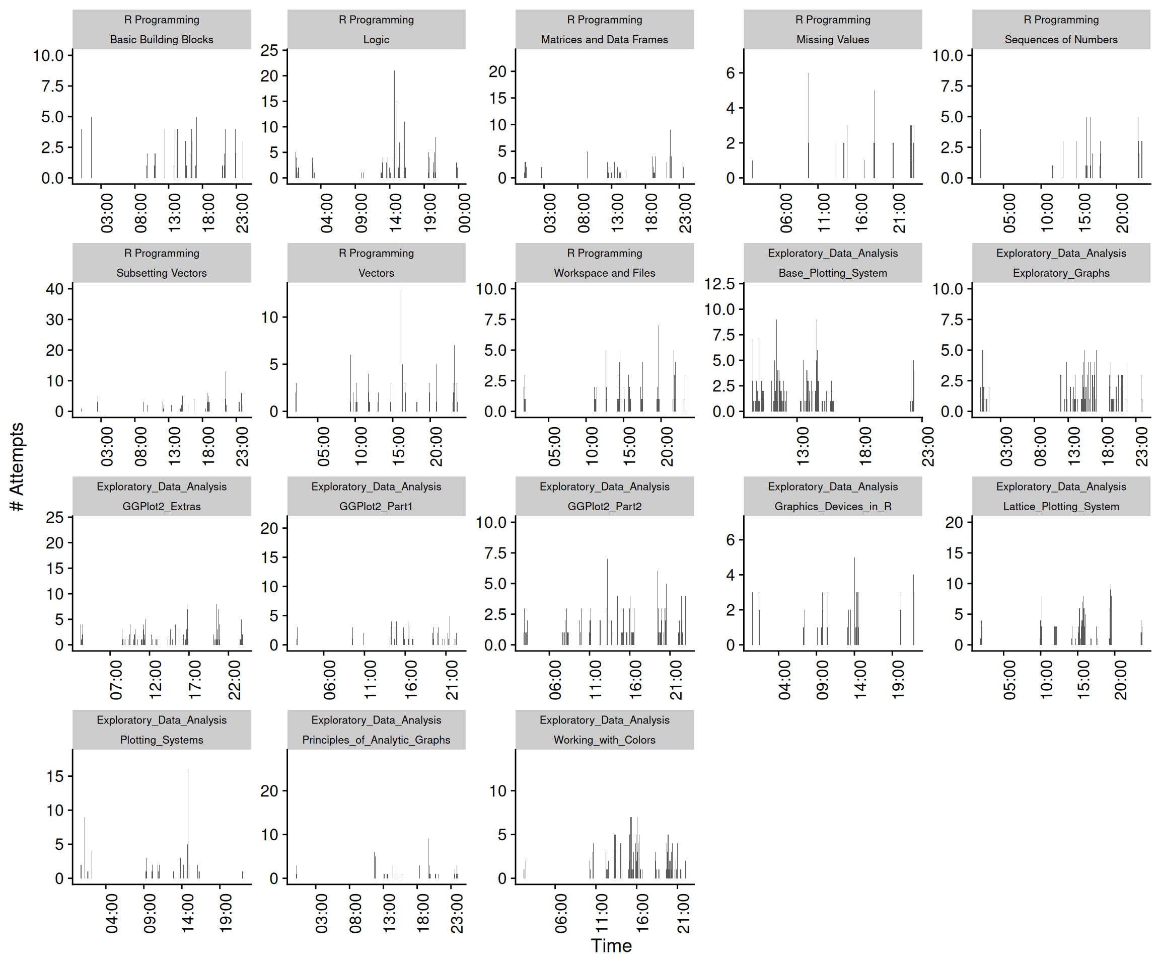
Assignment 1
#Filtering for Assignment 1 by course_name
assign_1 = data |> filter(course_name == 'R Programming')
#Attempts by Question for each course-lesson
assign_1 |>
ggplot(aes(x=question_number, y=attempt)) +
geom_col() +
facet_grid(~lesson_name, scales='free_x') +
theme_cowplot() +
theme(strip.text.x = element_text(size = 8)) +
labs(x='Q #', y='# Attempts')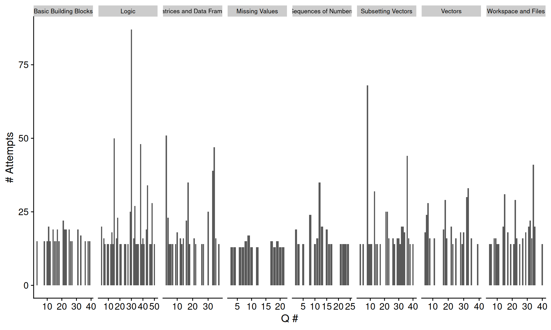
#Students struggled with questions in Logic, subsetting vectors, and matrices and dfs##Average of attempts for each lesson of each Assignment
lesson_counts_1 <- assign_1 |> count(lesson_name, question_number, student_id)
lesson_counts_1$question_number = as.factor(lesson_counts_1$question_number)
lesson_avgs_1 <- lesson_counts_1 %>% select(-c(student_id)) %>% group_by(lesson_name, question_number) %>% summarise(avg = mean(n))
##Compare for all lessons
lesson_avgs_1 |>
ggplot(aes(x=lesson_name, y=avg)) +
geom_boxplot(alpha = 0.5) +
geom_jitter() +
theme_cowplot() +
theme(axis.text.x = element_text(angle=90, hjust=1), strip.text.x = element_text(size = 8)) +
labs(y='Avg Attempts', x='Lesson')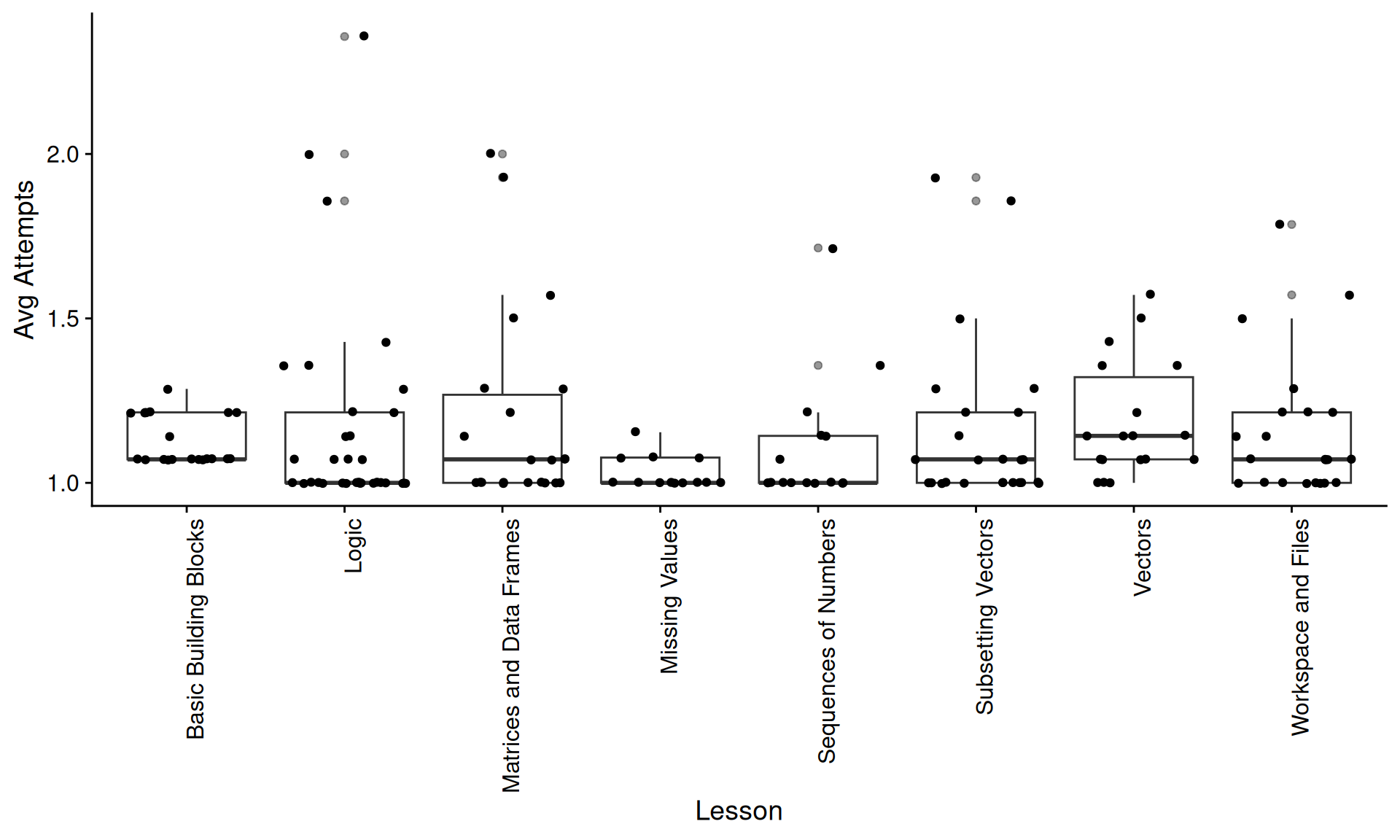
#Higher average attempts in lessons from logic, matrices and dfs, subsetting vectors
#Understandable new data structures they are getting familiar with and logical thinking
#Looking at dates completed
assign_1 |>
ggplot(aes(x=date, y=attempt)) +
geom_col() +
facet_grid(~lesson_name, scales='free_y') +
theme_cowplot() +
theme(axis.text.x = element_text(angle=90, hjust=1), strip.text.x = element_text(size = 8)) +
labs(x='Date', y='# Attempts')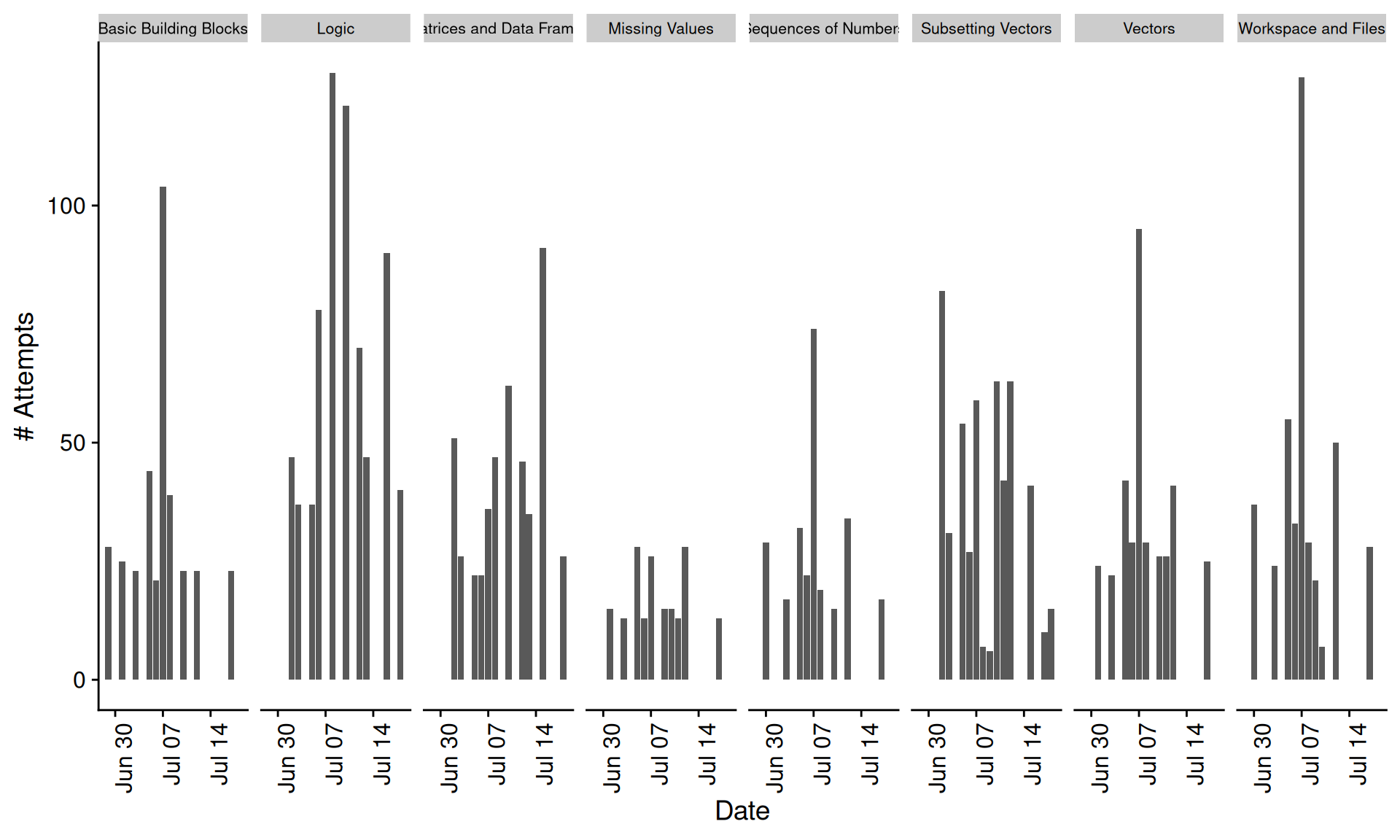
#Calendar Heatmap
calendar_df_1 <- assign_1 %>% count(date)
days_1 <- calendar_df_1$n
days_1 <- c(days_1, rep(0,14))

calendR(from = "2025-06-29",
        to = "2025-07-30",
        special.days = days_1,
        gradient = TRUE,
        low.col = "white",
        special.col = "#FF0000")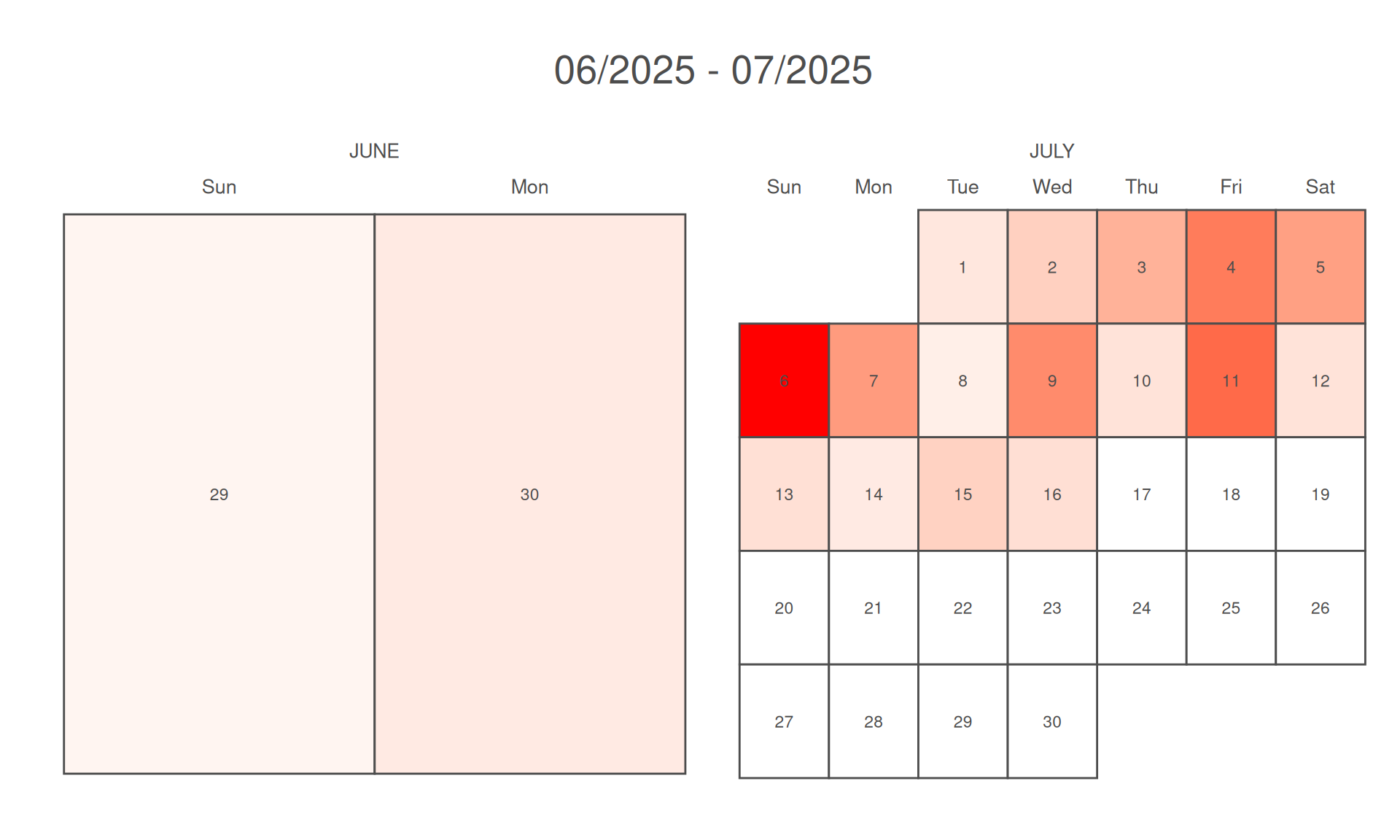
#Busiest submission date was 2 days before! Nice early birds!#Looking at time of completion for each lesson
assign_1 |>
ggplot(aes(x=as.POSIXct(time, format="%H:%M"), y=attempt)) +
geom_col() +
scale_x_datetime(
date_breaks = "2 hour",
date_labels = "%H:%M") +
theme_cowplot() +
theme(axis.text.x = element_text(angle=90, hjust=1), strip.text.x = element_text(size = 8)) +
labs(x='Time', y='# Attempts')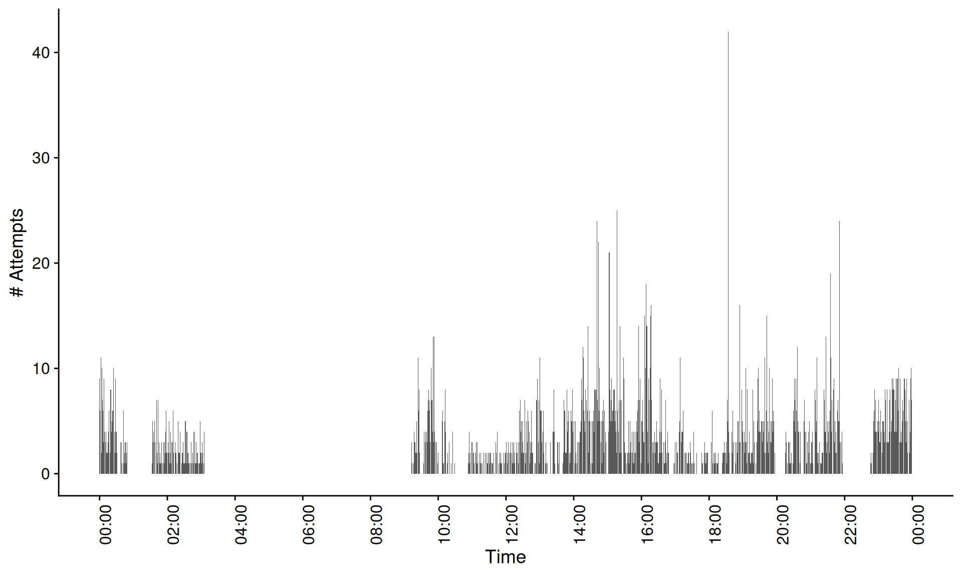
# Evening submissions are popular, some early risers among us Assignment 2
#Filtering for Assignment 2
assign_2 = data |> filter(course_name == 'Exploratory_Data_Analysis')
#Attempts by Question for each course-lesson
assign_2 |>
ggplot(aes(x=question_number, y=attempt)) +
geom_col() +
facet_grid(~lesson_name, scales='free_x') +
theme_cowplot() +
theme(strip.text.x = element_text(size = 8)) +
labs(x='Q #', y='# Attempts')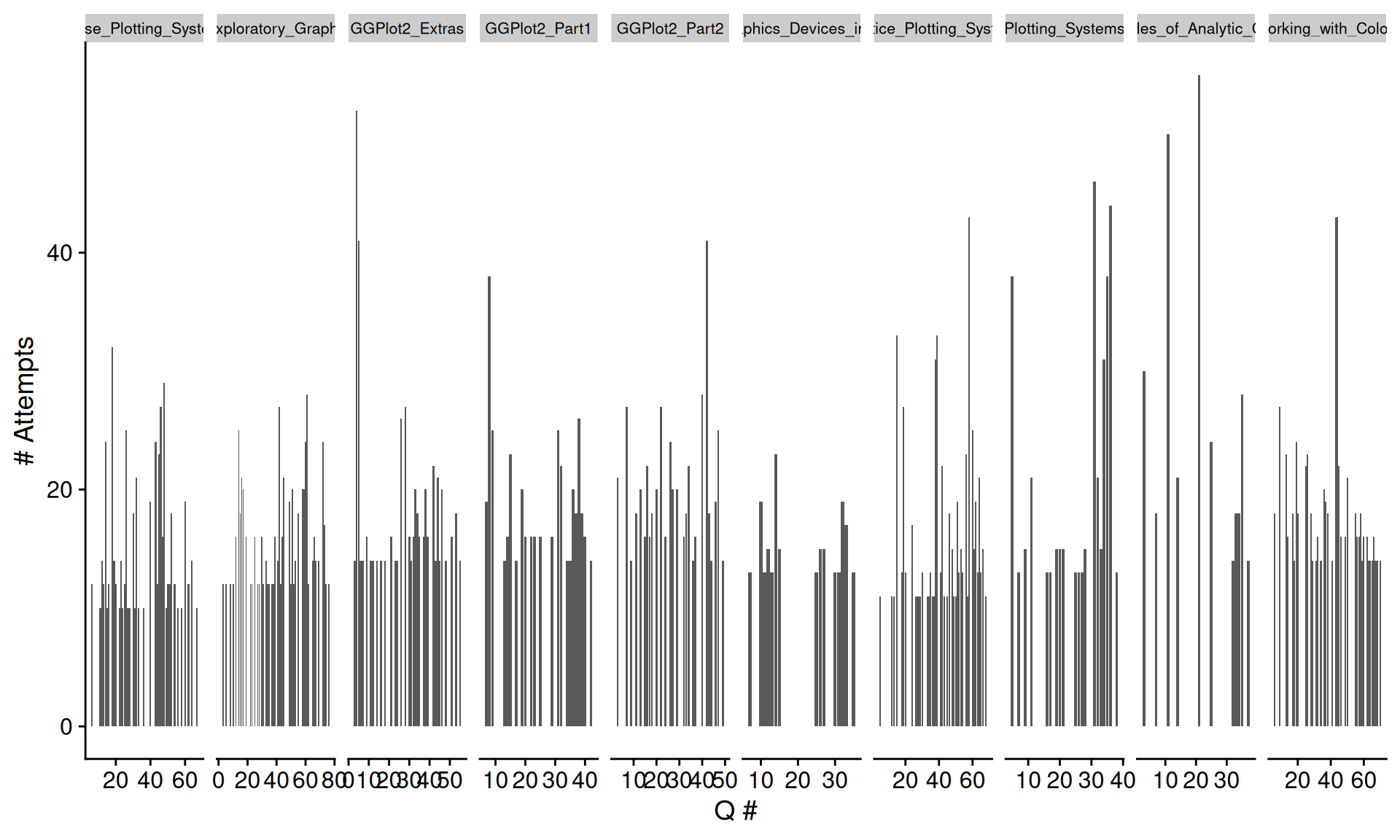
#High number of attempts in plotting systems lessons and principles of analyti graphs##Average of attempts for each lesson of Assignment
lesson_counts_2 <- assign_2 |> count(lesson_name, question_number, student_id)
lesson_counts_2$question_number = as.factor(lesson_counts_2$question_number)
lesson_avgs_2 <- lesson_counts_2 %>% select(-c(student_id)) %>% group_by(lesson_name, question_number) %>% summarise(avg = mean(n))
##Compare for all lessons
lesson_avgs_2 |>
ggplot(aes(x=lesson_name, y=avg)) +
geom_boxplot(alpha = 0.5) +
geom_jitter() +
theme_cowplot() +
theme(axis.text.x = element_text(angle=90, hjust=1), strip.text.x = element_text(size = 8)) +
labs(y='Avg Attempts', x='Lesson')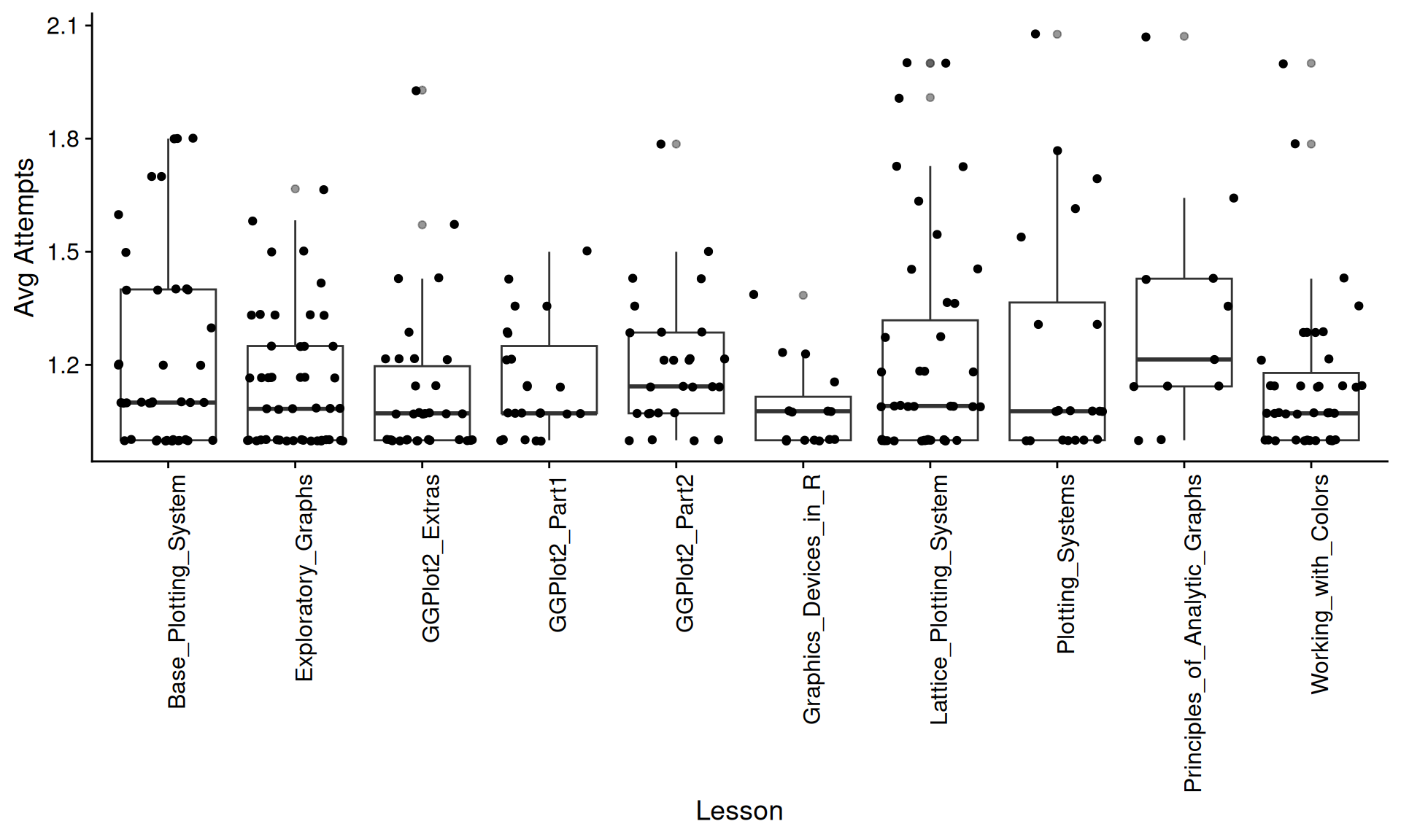
#Not that high of an average per lesson #Calendar Heatmap
calendar_df_2 <- assign_2 %>% count(date)
days_2 <- calendar_df_2$n
days_2 <- c(rep(0,7), days_2, rep(0,7))
calendR(from = "2025-07-01",
to = "2025-07-30",
special.days = days_2,
gradient = TRUE,
low.col = "white",
special.col = "#FF0000")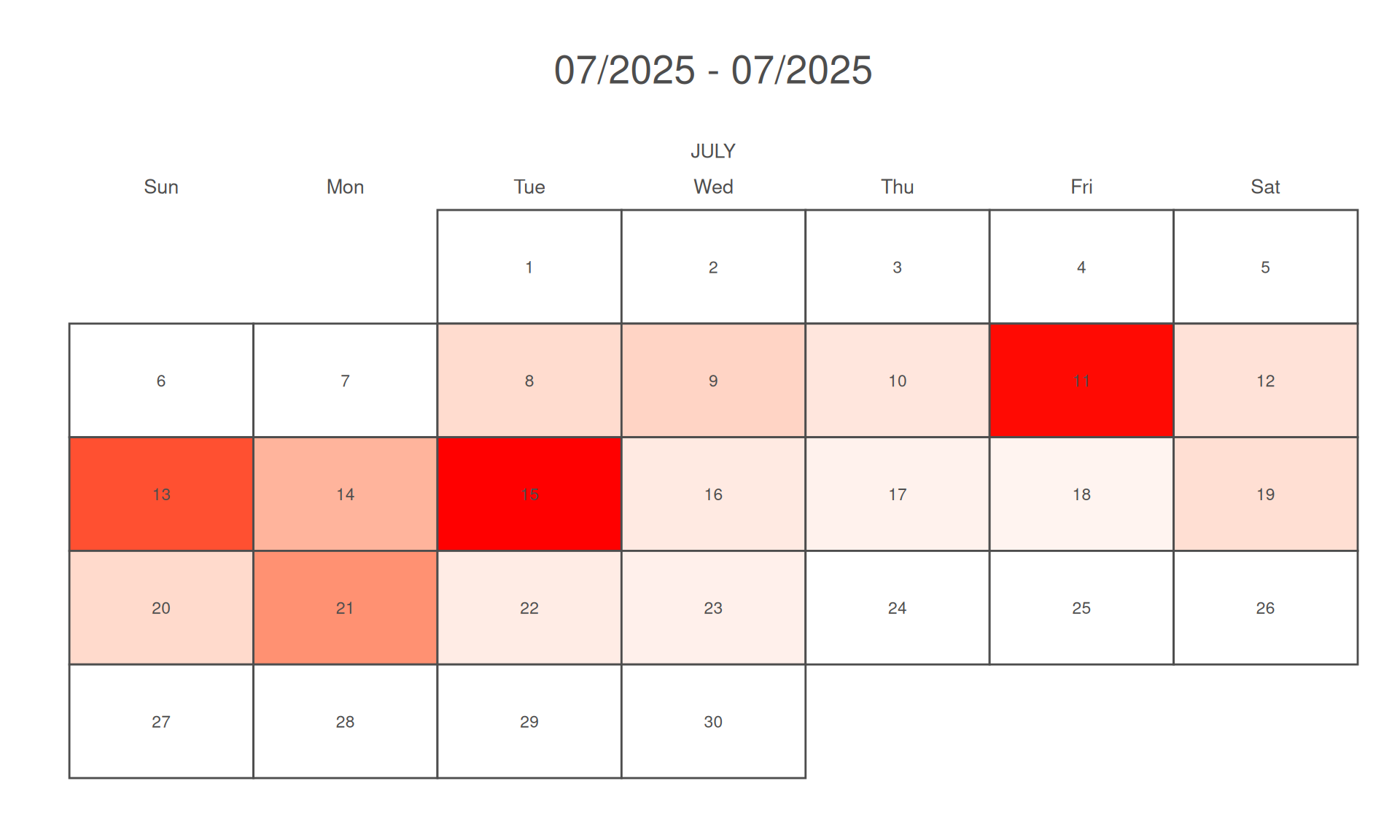
# High submission dates early and on day of soft due date#Looking at time of completion for each lesson
assign_2 |>
ggplot(aes(x=as.POSIXct(time, format="%H:%M"), y=attempt)) +
geom_col() +
scale_x_datetime(
date_breaks = "5 hour",
date_labels = "%H:%M") +
theme_cowplot() +
theme(axis.text.x = element_text(angle=90, hjust=1), strip.text.x = element_text(size = 8)) +
labs(x='Time', y='# Attempts')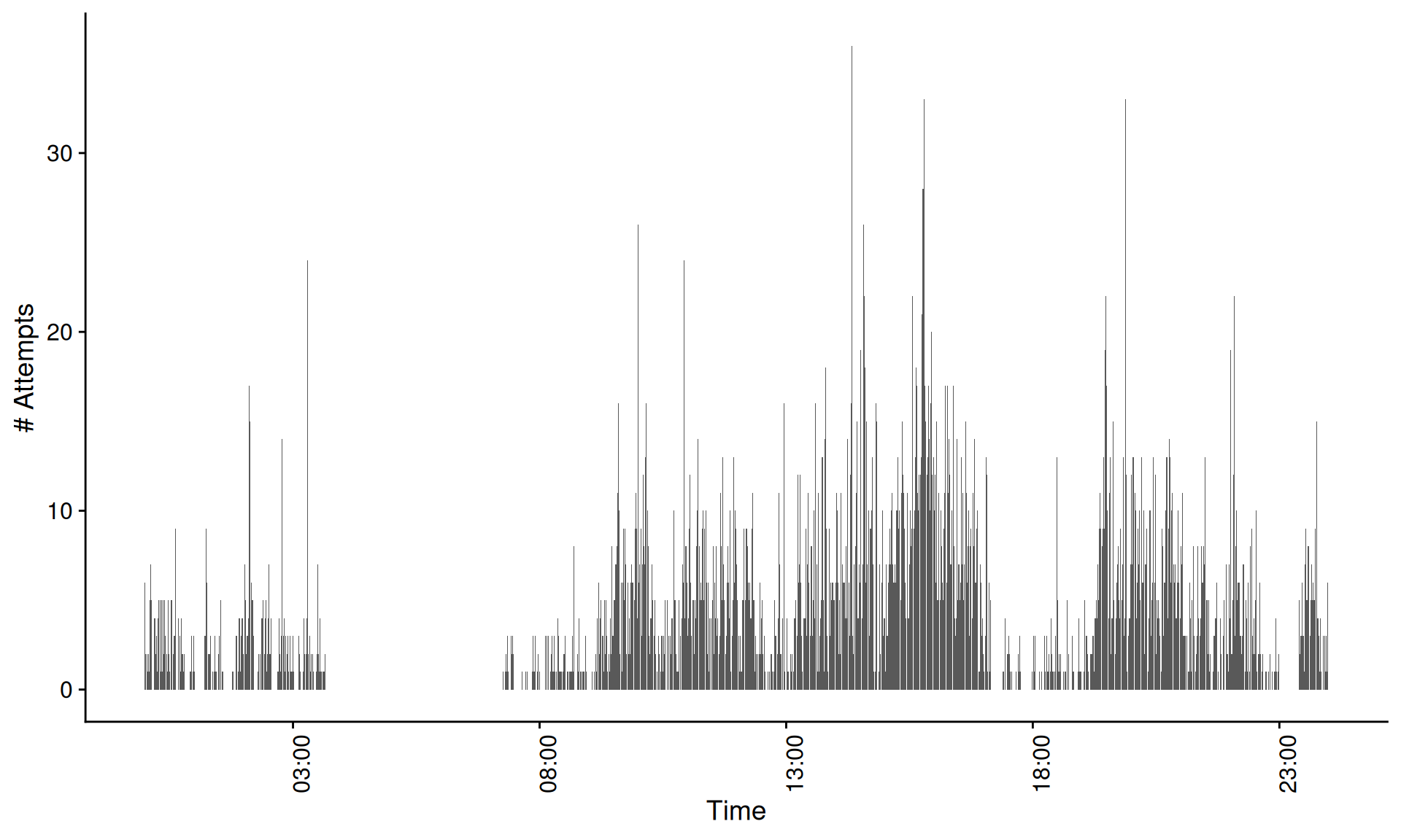
#Some students are up very late, but most work in the evening after hours